Optimizers in PyPose - Gauss Newton and Levenberg-Marquadt

July 14, 2023SLAMRobotics

In deep learning, we usually use first-order optimizers like Stochastic Gradient Descent, Adam, or RMSProp.

However, in SLAM problems, we use Bundle Adjustment to jointly optimize camera pose and landmark coordinate in real time. Naive first order optimizers is not efficient enough (requires many iterations to converge) for this situation.

In this post, I will introduce the concept of second order optimizer. However, since the second order optimizer requries us to derive the Hessian matrix for the optimization target, it is usually impractical to use it directly. Therefore, we will use the Gauss-Newton and Levenberg-Marquadt optimizers instead.

Optimization Problem

The optimization problem, in general can be represented in the form of

x^* = \arg\min_{x}f(x)

That is, we want to find some optimal input $x^*$ s.t. such input can minimize some given expression $f(x)$ .

Naive Optimization

When function $f$ is simple, we can find its Jacobian matrix (first order derivative) $\mathbf{J}$ and Hessian matrix (second order derivative) $\mathbf{H}$ easily.

\mathbf{J} = \begin{bmatrix} \frac{\partial f}{\partial x_0} & \frac{\partial f} {\partial x_1} & \cdots & \frac{\partial f}{\partial x_n} \end{bmatrix} \quad \mathbf{H} = \begin{bmatrix} \frac{\partial^2 f}{\partial x_1^2} & \frac{\partial^2f}{\partial x_1 \partial x_2} & \cdots & \frac{\partial^2 f}{\partial x_1\partial x_n} \\ \frac{\partial^2 f}{\partial x_2\partial x_1} & \frac{\partial^2 f}{\partial x_2^2} & & \vdots \\ \vdots & & \ddots & \vdots \\ \frac{\partial^2 f}{\partial x_n\partial x_1} & \cdots & \cdots & \frac{\partial^2 f}{\partial x_n^2} \end{bmatrix}

We can then solve for $\mathbf{J}x = \mathbf{0}$ . For every solution $x$ , if the hessian matrix is positive definite, then a local minimum is found.

Iterative Optimization

However, when the function $f$ is complex or $x$ lives in very high dimension (~10k in sparse 3D reconstruction problem, or ~10M in usual neural network models), it is practically impossible to solve for analytical solution of $\mathbf{J}$ and $\mathbf{H}$ .

In this case, we need to use iterative optimization. The general algorithm for such approach can be summarized as following:

For some initial guess value $x_0$ , we have $x \gets x_0$
While true
1. Use the Taylor expansion of $f$ around $x$ ,
  
  If using second-order optimizer, we have
  $\hat{f}(x + \Delta x) = f(x) + \mathbf{J}(x)\Delta x + \frac{1}{2}\Delta x^T\mathbf{H}(x) \Delta x$
  If using first-order optimizer, we have
  $\hat{f}(x + \Delta x) = f(x) + \mathbf{J}(x)\Delta x$
2. Solve for $\Delta x^*$ such that
$\Delta x^* = \arg\min_{\Delta x}{\hat{f}(x + \Delta x)}$
1. Update $x \gets x + \Delta x^*$
2. If $\|\Delta x^*\|_2 < \varepsilon$ , the solution "converges" and break out the loop
Return $x$

First Order Optimizers

When using first order optimizer, we only use the first order derivative of $f$ to calculate $\Delta x^*$ . Then, we have

\Delta x^* = \arg\min_{\Delta x} f(x) + \mathbf{J}(x) \Delta x = \arg\min_{\Delta x} \mathbf{J}(x) \Delta x = -\arg\max_{\Delta x}{\mathbf{J}(x) \Delta x}

Obviously, the solution will be $\Delta x^* = -\mathbf{J}(x)$ . This is aligned with the definition of naive Stochastic Gradient Descent (SGD).

Intuitively, we can interpret first order optimization as locally approximate the optimization target $f$ as a plane with form of $\mathbf{J}x$ .

20230723164733

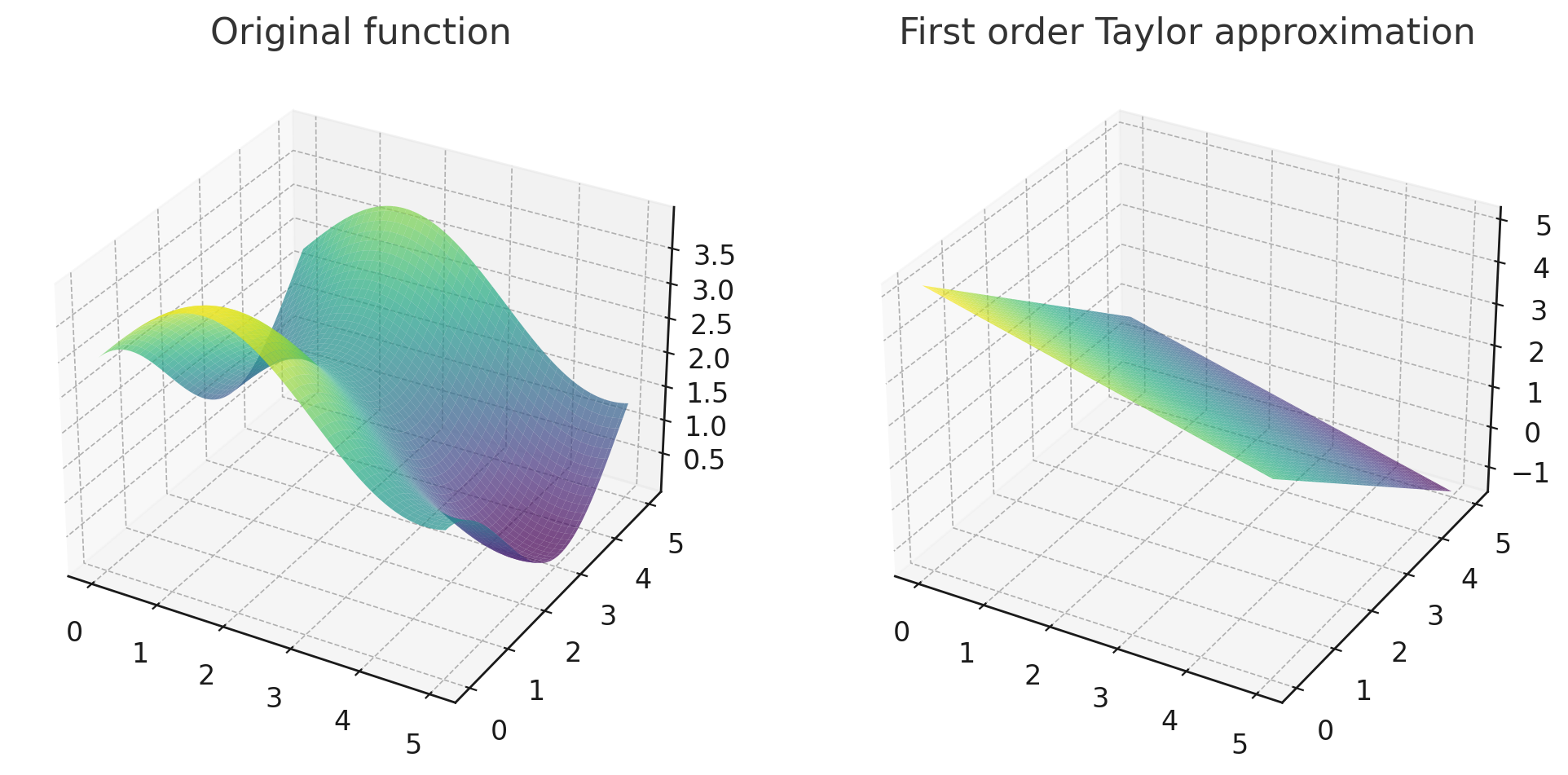
First order Taylor approximation of $\sin(x) + \cos(y) + 2$ at $(2, 2)$ . Generated by GPT-4 with code interpreter.

Such optimizer and its variants like Adam, AdamW, RMSProp are widely used in the field of deep learning and is supported by popular libraries like PyTorch.

Why not First Order Optimizer?

While first order optimizers can support large scale optimization problem, it generally requires more iterations to converge since linearization (first order Taylor expansion) is not a good approximation.

In applications like SLAM where bundle adjustments need to run in real-time, first order optimizer cannot fulfill our need.

Therefore, we have the second order optimizers.

Second Order Optimizers

The second order optimizers, specifically the Newton method uses second order Taylor expansion as the local approximation for optimization target:

\hat{f}(x + \Delta x) = f(x) + \mathbf{J}(x)\Delta x + \frac{1}{2}\Delta x^T \mathbf{H}(x) \Delta x

Then we have

\Delta x^* = \arg\min_{\Delta x}{\hat{f}(x + \Delta x)} = \arg\min_{\Delta x}\mathbf{J}(x)\Delta x + \frac{1}{2}\Delta x^T\mathbf{H}\Delta x

Solving

\frac{\partial }{\partial\Delta x} {\left(\mathbf{J}(x)\Delta x + \frac{1}{2}\Delta x^T\mathbf{H}\Delta x\right)} = \mathbf{0}

We have $\mathbf{H}(x)\Delta x^* = -\mathbf{J}(x)$ .

Intuitively, the second order optimizers like Newton method is using a paraboloid to locally approximate the function surface.

20230723164919

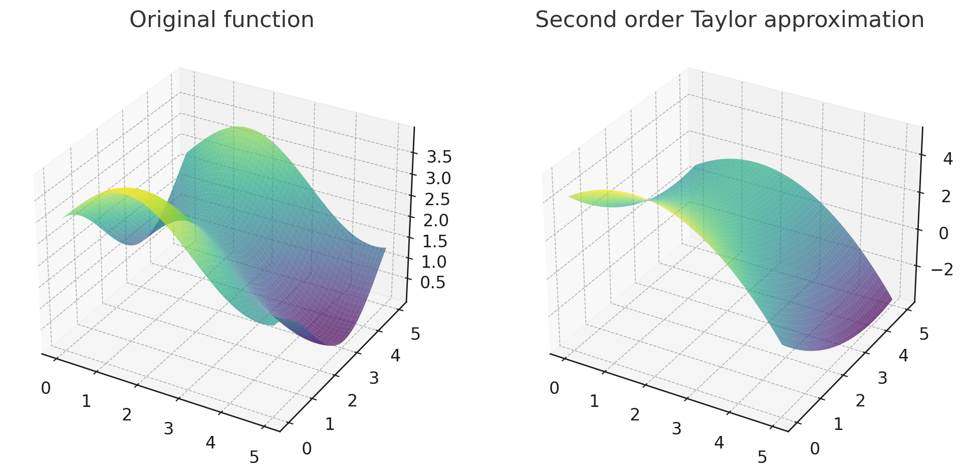
Second order Taylor approximation of $\sin(x) + \cos(y) + 2$ at $(2, 2)$ . Generated by GPT4 with code interpreter.

Why not Second Order Optimizer?

Second order optimizer provides a much better approximation to the original function. Hence, solver with second order optimizer can converge much faster than first order optimizer.

However, it is often not practical to calculate the $\mathbf{H}$ of $f$ . If $x \in \mathbf{R}^d$ , then $\mathbf{H}$ will have $d^2$ elements.

Pseudo-second-order Optimizers

Gauss-Newton Optimizer

Gauss-Newton optimizers requires the expression to be optimized to be in the form of sum-of-square. That is, the optimization target must have form of

\mathbf{R}(x) = \sum{f(x)^2}

Then, consider the first order approximation for $f$ at $x$ :

\hat{f}(x + \Delta x) \approx f(x) + \mathbf{J}(x) \Delta x

$\begin{aligned} \Delta x^* &= \arg\min_{\Delta x} \mathbf{R}(x + \Delta x)\\ &\approx \arg\min_{\Delta x}{(f(x) + \mathbf{J}(x)\Delta x)^2}\\ &= \arg\min_{\Delta x}{f^2(x) + 2f(x)\mathbf{J}(x)\Delta x + (\mathbf{J}(x)\Delta x)^\top (\mathbf{J}(x) \Delta x)}\\ \end{aligned}$

Since the term in $\arg\min$ is convex (is a square), we know the optimization target must be convex. Hence, we have $\Delta x = \Delta x^*$ when $\frac{\partial (f(x) + \mathbf{J}\Delta x)^2}{\partial \Delta x} = 0$ .

Hence, we have

\mathbf{J}^\top(x) \mathbf{J}(x) \Delta x^* = -f(x)\mathbf{J}(x)

where we can solve for $\Delta x^*$ .

Problem of Gauss-Newton Optimizer

In production environment, we may have $\mathbf{J}$ not full-ranked. This will cause the coefficient matrix $\mathbf{J}^\top \mathbf{J}$ on the left hand side being positive semi-definite (not full-ranked). In this case, the equation system is in singular condition and we can't solve for $\Delta x^*$ reliably.

Also, in Gauss-Newton method, the $\Delta x^\*$ we solved for may be very large. Since we only use the first order Taylor expansion, large $\Delta x^\*$ usually indicates a poor approximation for $f(x + \Delta x^\*)$ . In these cases, the residual $\mathbf{R}$ may even increase as we update $x \gets x + \Delta x$ .

Levenberg-Marquadt Optimizer

Levenberg-Marquadt optimizer is a modified version of Gauss-Newton optimizer.

The LM optimizer use a metric $\rho$ to evaluate the quality of approximation:

\rho(\Delta x) = \frac{f(x + \Delta x)}{f(x) + \mathbf{J}(x)\Delta x}

When the approximation is accurate, we have $\rho(\Delta x) = 1$ .

LM optimizer will then use this measure of approximation quality to control the "trusted region". The "trusted region" represents a domain where the first order approximation for $f(x)$ is acceptable.

The update vector $\Delta x$ must be in the trusted region. Hence, the entire optimization problem is formulated as

\arg\min_{\Delta x}{(f(x) + \mathbf{J}(x)\Delta x)^2} \quad \text{s.t. }D\Delta x \leq \mu

where $D$ is a diagonal matrix constraining the $\Delta x$ in an ellipsoid domain.

Usually, the $D$ is configured as $diag(\mathbf{J}^\top(x)\mathbf{J}(x))$ . This allows the update step to move more on the direction with lower gradient.